A Pivot Table is brilliant at summarising your data, but even a good one is still a table full of numbers that takes a moment to read. A Pivot Chart takes that same summary and turns it into a proper chart, so whoever’s looking at it gets the story instantly.
Building one
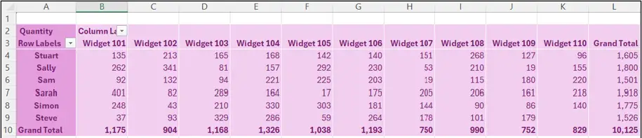
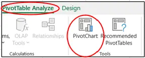
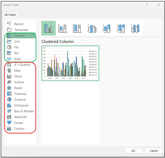
Click anywhere on an existing Pivot Table, go to the PivotTable Analyze ribbon, and select PivotChart. You’ll see a list of chart types to choose from, though a handful of the more specialist styles (Scatter, for example) aren’t available from Pivot Table data, so the list is a little shorter than the full chart menu. Pick whichever style fits what you’re trying to show and click OK.
Once it’s created, the field list changes slightly, Columns becomes Legend (Series) and Rows becomes Axis (Categories), but don’t let the terminology put you off, it’s still the same simple drag and drop you used to build the Pivot Table in the first place.
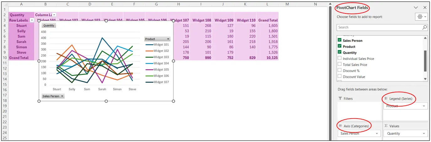
They’re properly linked
A Pivot Chart and its Pivot Table share the exact same underlying data, they’re really the same entity just displayed differently. Change a field on the chart and the table updates too, and vice versa, it’s impossible for one to show something the other doesn’t. The chart has to live in the same file as its table, though it doesn’t need to sit on the same sheet.
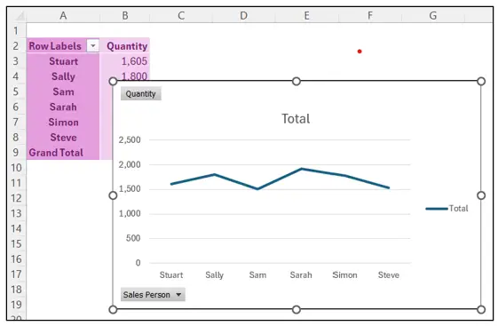
Top Tip: cut and paste several Pivot Charts onto their own sheet to build yourself a dashboard.
Refreshing and formatting
Right click either the table or the chart and choose Refresh Data, and both update together, along with anything else connected to the same source data.
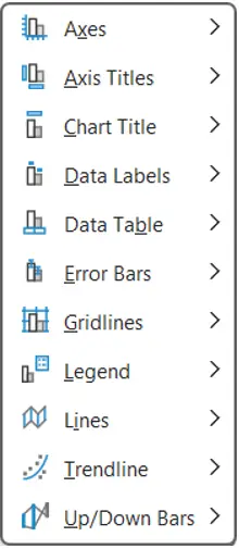
For formatting, the Design ribbon gives you a set of preset Styles, Change Colours lets you pick a different palette, and Add Chart Element lets you add or remove things like the legend and data table.


I usually remove the little grey field buttons that appear by default, purely a personal preference, done from PivotChart Analyze, Field Buttons.
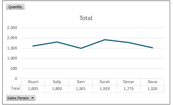
Bonus Tip: once you’ve formatted one Pivot Chart the way you like it, click its outside edge, copy it, then paste that formatting straight onto another Pivot Chart, no need to start from scratch each time.
Worth knowing
You can also create a Pivot Chart directly from raw data without building the Pivot Table first, Excel will simply create both at once, since you can’t really have one without the other.
The trade off is you lose access to a few of the fancier chart formats available with standard charts, but for most reporting, the ability to drag and drop fields exactly where you need them usually wins out.