We’re all used to writing a formula, pressing enter, then copying it down rows or across columns, over and over. In modern versions of Excel (Microsoft 365), there’s a genuinely better way to manage this: Dynamic Arrays. Write one single formula in one cell, press Enter, and Excel instantly spills the results into all the neighbouring cells that are needed, no dragging, no copying, and it automatically expands or shrinks as your data changes. This is what I’d call ACE.
The functions worth knowing first
UNIQUE() returns every distinct value from a list instantly, brilliant for pulling a clean list of customers, suppliers or codes with none of the manual duplicate removal that used to be needed.
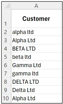
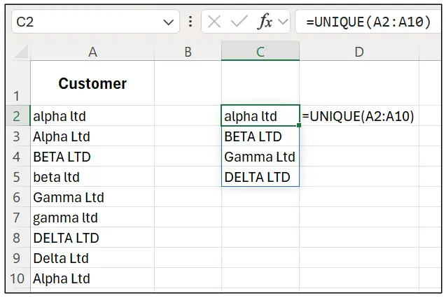
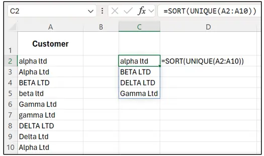
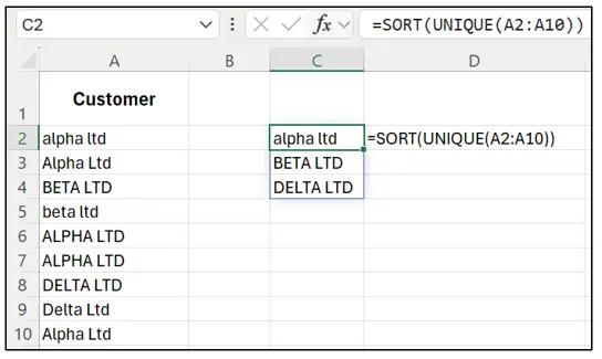
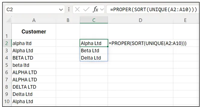
SORT() arranges a list into order dynamically, and wrapping it around UNIQUE like =SORT(UNIQUE(A2:A10)) gives you a clean, alphabetically sorted list of unique values in one single formula. Add PROPER() around the outside too and you can tidy up inconsistent capitalisation at the same time.
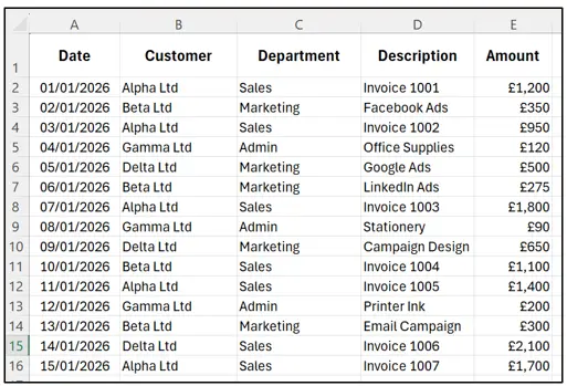
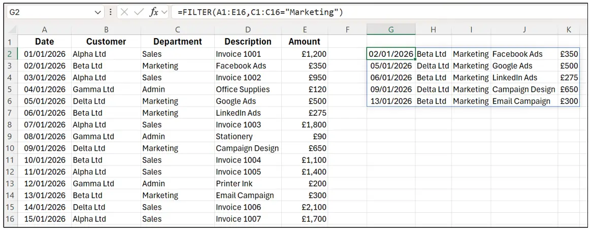
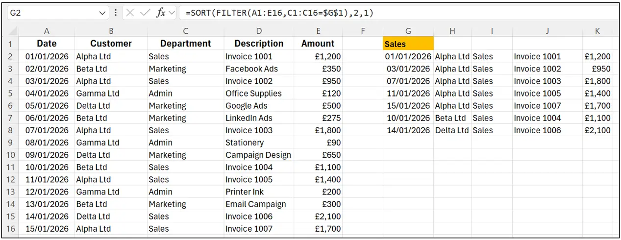
FILTER() returns only the rows that meet a condition you set, for example =FILTER(A1:E16,C1:C16=”Marketing”) pulls every row relating to Marketing with no manual filtering or copying required, and your original data stays completely untouched.
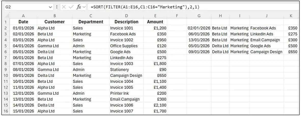
You can wrap SORT around a FILTER too, to sort the results by whichever column you choose.
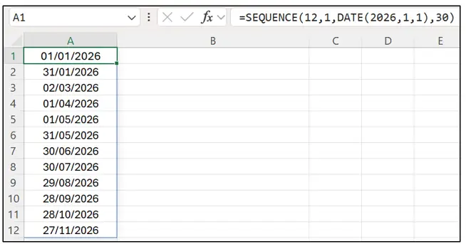
SEQUENCE() generates a list of numbers or dates in one go, useful for building reporting periods or invoice numbers without dragging a fill handle down a column.
Combining them for something genuinely powerful
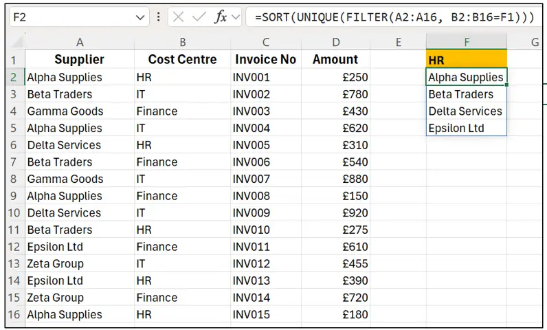
The real magic happens when you stack these together, for example:
=SORT(UNIQUE(FILTER(A2:A16,B2:B16=F1)))
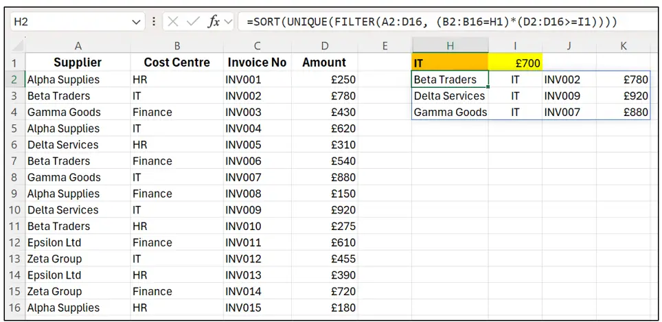
filters your data down to a specific selection, removes duplicates, sorts the result, and updates automatically the moment anything changes. One formula replacing what used to be several manual steps, or a Pivot Table, depending on what you needed.
A couple of practical notes
Dynamic Arrays work in Microsoft 365 and Excel Online (I also wrote about them for Executive Support Magazine) (not in older perpetual versions), and they play especially nicely with Excel Tables, for example =UNIQUE(Table1[Customer]) instead of a fixed cell range.
If a formula tries to spill into cells that already contain data, you’ll see a #SPILL! error, Excel simply doesn’t have anywhere to put the results. Clear whatever’s in the way and the formula will spill exactly as expected.
Start simple
Try =UNIQUE(A:A) on your own data today, and build up to combining functions as your confidence grows. Once you see how much manual tidying up one Dynamic Array formula can replace, it’s genuinely hard to go back to copying formulas down a column the old way.