VLOOKUP is one of the most widely used formulas in Excel, and also one of the most commonly muddled up, mostly because the four pieces of information it needs are easy to mix up if you haven’t written many of them.
What it actually does
VLOOKUP searches for a value in the first column of a range and returns a value from another column on that same row.
In plain terms, you give it something to search for, tell it where to search, and tell it what to bring back. VLOOKUP stands for Vertical Lookup, since it works down columns, there’s also a lesser used HLOOKUP for horizontal data, and it’s just as ACE, simply not needed as often. There is also a new swanky XLOOKUP too…….watch out for that coming soon in a later blog post.
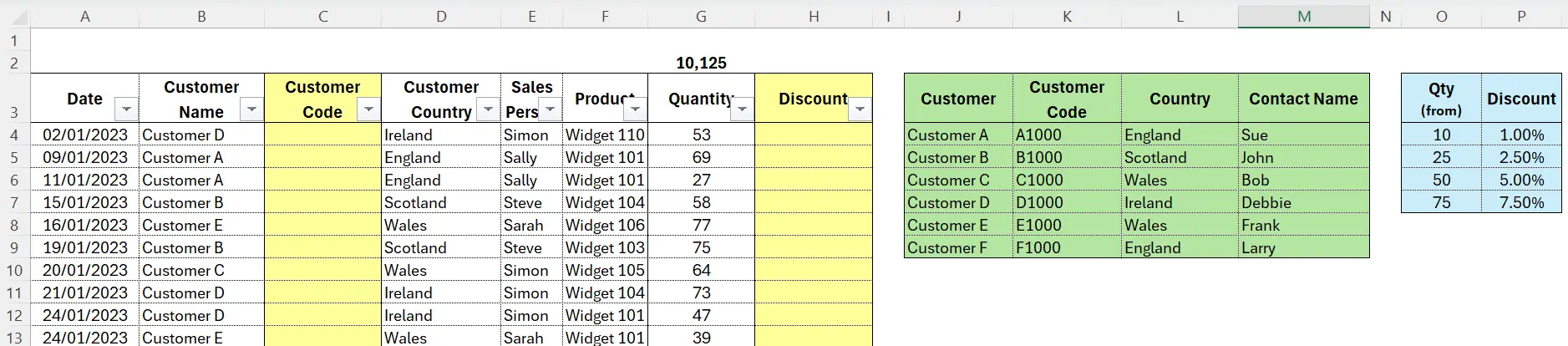
The four parts
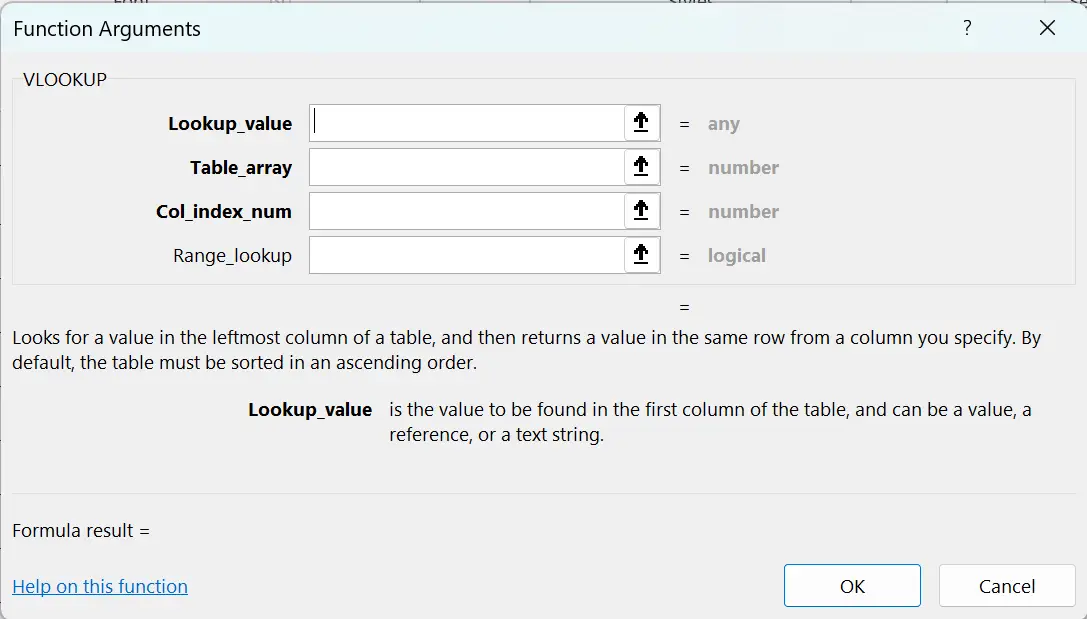
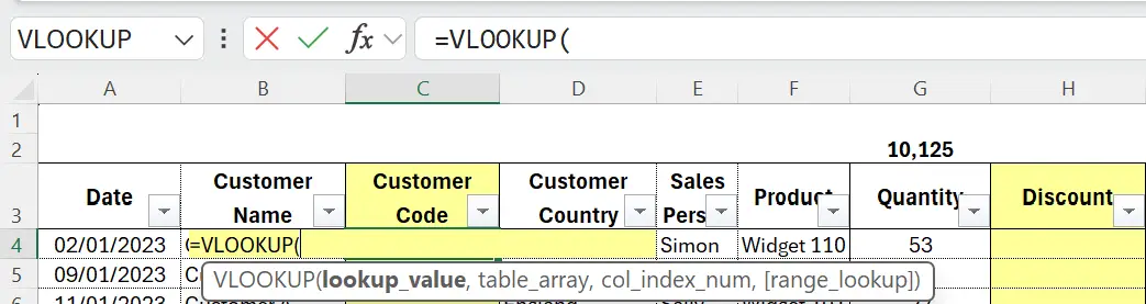
The formula is written as
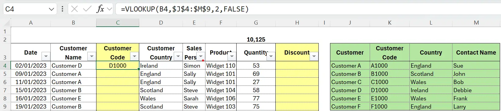
=VLOOKUP(lookup_value, table_array, col_index_num, range_lookup).
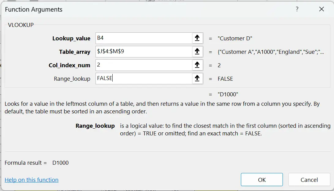
lookup_value is what you’re searching for
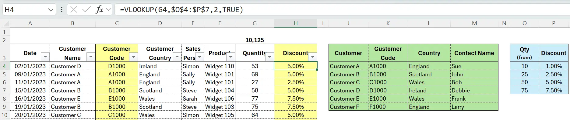
table_array is the range to search AND return from (freeze it with $ signs so it doesn’t shift when you copy the formula)
col_index_num is which column in that range to return, counting from the first column of your chosen range, not from the start of the whole sheet
range_lookup decides whether you want an exact match (FALSE) or the nearest match (TRUE, which requires the data to be sorted first).
The do’s and don’ts
- Do make sure the value you’re searching for exists in the FIRST column of your chosen range, VLOOKUP can only search left to right.
- Do specify FALSE for exact matches, particularly with text or codes.
- Do double check your column number, it won’t update automatically if columns are inserted or deleted.
- Don’t forget to freeze your table reference with $ if you’re copying the formula down or across.
- Don’t overlook trailing spaces, VLOOKUP can’t find a match if there’s an invisible space at the end of your text, wrap the lookup value in TRIM() to fix it.
Where it falls down
VLOOKUP only searches left to right, so if the column you want to return sits before your lookup column, it simply won’t work.
It’s not case sensitive, so it treats ABC and abc as identical, and performance can slow down noticeably on bigger datasets.
When it can’t find a match it returns an unsightly #N/A, so it’s often paired with IFERROR to return something more useful instead.
If any of that sounds like a dealbreaker, XLOOKUP (or INDEX and MATCH combined) solves most of VLOOKUP’s limitations, worth knowing about even if VLOOKUP remains your everyday go to.
Used properly though, VLOOKUP is genuinely one of the most useful tools in your Excel toolkit, and once the four arguments click, you’ll wonder how you managed without it.