Raw data in a spreadsheet can be genuinely hard to make sense of at a glance, and this is exactly where Conditional Formatting earns its keep (I first wrote about it as a way to become a trend spotter). Instead of manually colouring cells to flag what matters, you set a rule once and Excel keeps applying it automatically, updating instantly as your data changes.
A simple target example
Say you’ve got a column of sales figures and a target of £5,000. Select the column, go to Home, Conditional Formatting, Highlight Cell Rules, Greater Than, and enter your target. Every figure that beats it lights up straight away.
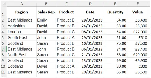

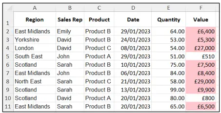
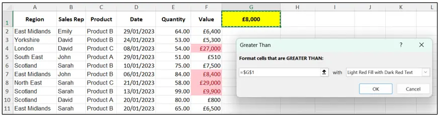
Pro tip: instead of typing 5000 directly into the rule, reference a cell containing your target instead, that way when the target changes, your formatting updates with it automatically, which is a much simpler way to control your spreadsheet.
Flagging overdue deadlines
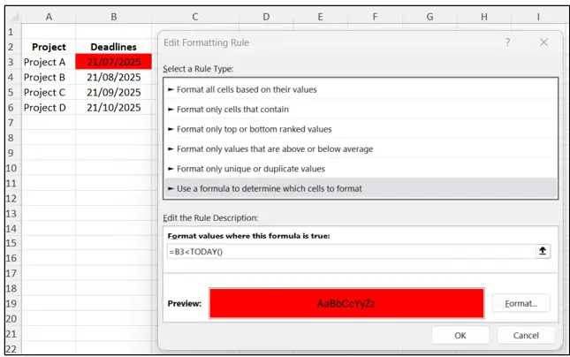
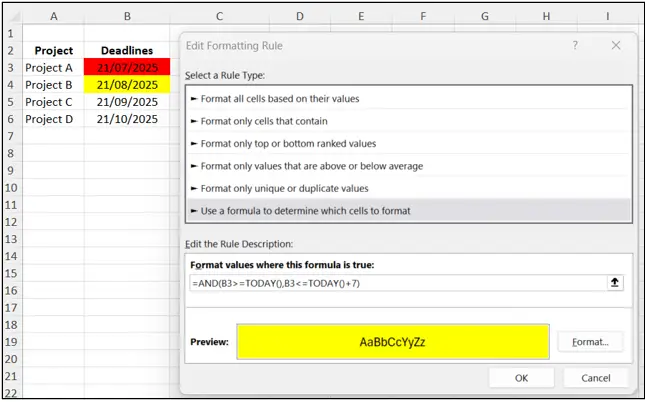
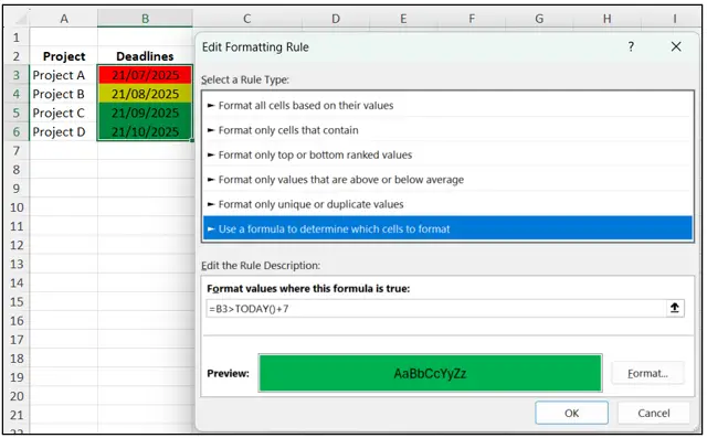
For anything date based, a formula based rule is the way to go.
Using Home, Conditional Formatting, New Rule, Use a Formula, you could set:
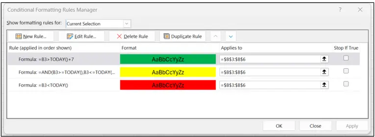
=B3<TODAY() for anything overdue (Red)
=AND(B3>=TODAY(),B3<=TODAY()+7) for anything due within a week (Amber)
=B3>=TODAY() for anything not yet due (Green),
Because it’s built on TODAY(), it recalculates every single day without you touching it, so nothing gets missed.
Spotting trends and duplicates
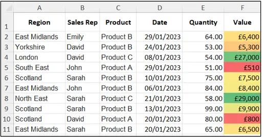
Colour Scales are brilliant when you’re not looking for a yes or no answer but a pattern across a whole column, the highest values shade green, the lowest red, and everything else grades in between, turning what could be hours of scanning into something obvious in seconds.
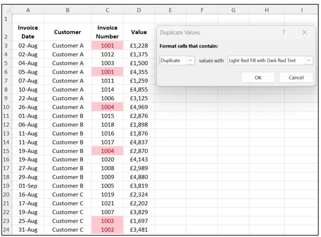
Highlighting Cell Rules, Duplicate Values does exactly what it says too, genuinely handy for spotting repeated invoice numbers or customer IDs that would be almost impossible to catch by eye.
Icon Sets, my personal favourite
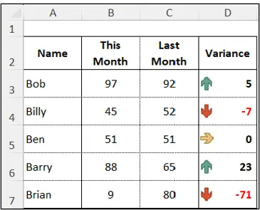
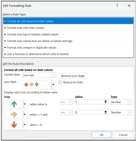
Sometimes a small icon communicates more clearly than colour ever could, a green arrow for improvement, amber for no change, red for decline.
Home, Conditional Formatting, Icon Sets, creates this in seconds, and it reduces a complex report down to a simple up, down, steady summary anyone can read instantly.
Formula driven rules, for more complex logic
You can base a rule on several conditions at once, for example sales below £8,000 AND region equal to Scotland, using a formula like:
=AND($F2<8000,$A2=”Scotland”)
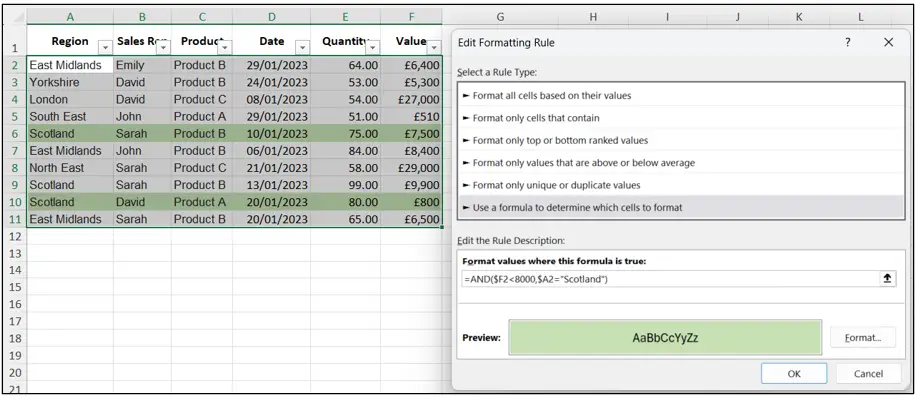
Conditional Formatting doesn’t need an IF wrapped around it either, the rule itself does the comparing.
Keeping it under control
Conditional Formatting is powerful, but it can get messy fast if you’re not careful. Keep it simple and only highlight what genuinely matters, use consistent colours across your files, and check the Rule Manager (Conditional Formatting, Manage Rules) regularly to avoid duplicate or conflicting rules, which can easily happen when copying and pasting formatted ranges. Think of it like a highlighter pen, if you highlight everything, nothing actually stands out.
So next time you’re staring at a daunting spreadsheet, ask yourself what you really need to see, and let Conditional Formatting do the heavy lifting for you.